Leapfrog and Minkowski's Question Mark Distribution
A Game of Leapfrog
Consider the following random process.
There are 3 frogs on a number line, initially at positions 0, 1, and 2. Every second, a random frog jumps over a random other frog. When a frog at position \(p\) (the “jumper”) jumps over a frog at position \(q\) (the “jumpee”), its new position becomes \(p+2(q-p)\); that is, the jumper maintains the same distance from the jumpee but lands on the opposite side.
At any given time, say the frogs are at positions \(p_1 \leq p_2 \leq p_3\). We define their aspect ratio to be \((p_2-p_1)/(p_3-p_1)\).
In the example above, the frogs start at \(\{0, 1, 2\}\). In the first move, the frog at \(1\) jumps over the frog at \(0\), resulting in \(\{-1, 0, 2\}\). In the next move, the frog at \(0\) jumps over the frog at \(2\), resulting in \(\{-1, 2, 4\}\), and so on. After 6 moves, the frogs are at \(\{-6, 1, 6\}\), so the aspect ratio at this step is \(\frac{7}{12}\).
Question:
What is the limiting distribution of this aspect ratio, as the number of moves goes to infinity?
I’ll guarantee you that this limiting distribution exists: there is some distribution \(X\) over \([0, 1]\) such that the distribution of the aspect ratio after \(n\) moves gets arbitrarily close in Earth mover’s distance to \(X\) for sufficiently large \(n\).
If you like doing these types of math problems, give it a try before reading on! If not, I’d encourage you to at least make a guess at the type of distribution you’re expecting. Is it uniform over \([0, 1]\)? Concentrated towards \(1/2\)? Is it discrete or continuous?
I’ll leave some empty space below to prevent spoilers.
Solution
It turns out that the limiting distribution looks like this:
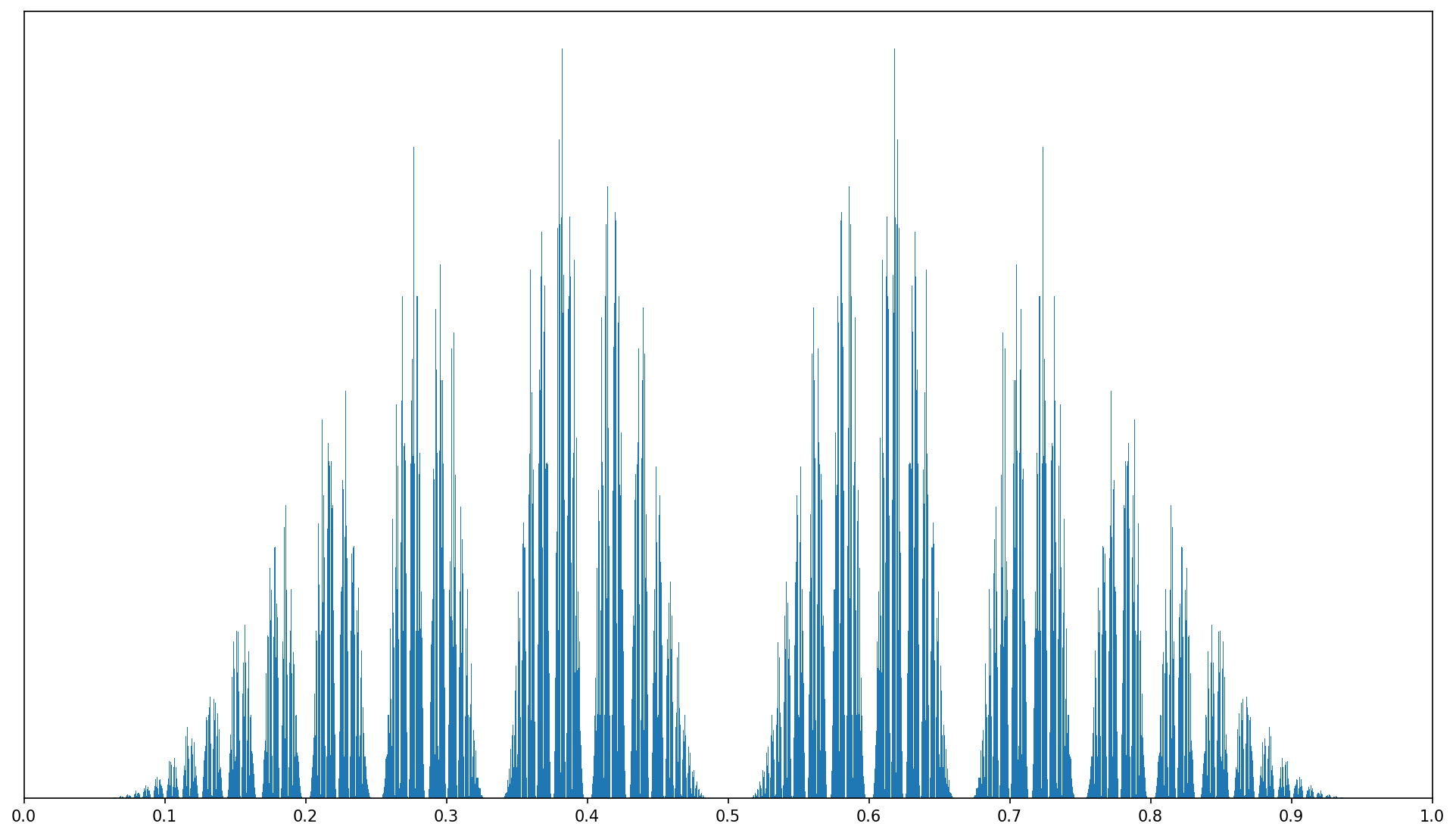
Pretty cool, right? If you study the distribution, you may notice that there is no probability mass around \(\frac{1}{2}\) or \(\frac{1}{3}\) or \(\frac{1}{4}\)… In fact, it seems like every rational number has an empty space around it. Meanwhile, one of the highest peaks of the distribution occurs at \(0.618\dots\), which some readers may recognize as the golden ratio \(\varphi\), also known as the “most irrational” number.
When I first considered this problem in 2023, I had no idea how to prove that the distribution looked like this — the best I could do was make an empirical simulation. Yet I was so intrigued by the fractally shape of the distribution that it has been my Twitter/X background image ever since:
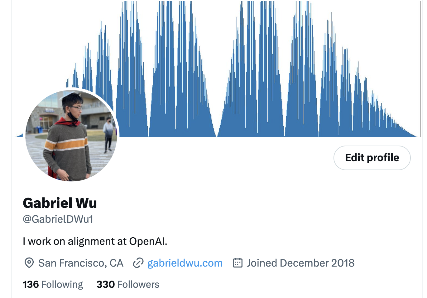
There are some small differences between this image (generated two years ago) and the one above (generated today), probably due to a small bug in my old code.
I gave the problem another try a few weeks ago. This time I found a simple way of understanding the distribution which I consider quite elegant, prompting this post.1 Like many other posts on this blog, the approach involves transforming one random process into an “isomorphic” one that is easier to understand.
Step 1: Exploiting Symmetries
If \(x\) is the aspect ratio, let the “symmetrized” aspect ratio be \(\min(x, 1-x)\). By symmetry, the distribution of the aspect ratio is equivalent to the distribution of the symmetrized aspect ratio reflected about \(1/2\) with probability \(1/2\).
Let’s modify the random process such that between every jump, we flip the entire diagram with probability \(1/2\), converting the aspect ratio \(x\) into \(1-x\) (call this a ‘flip operation’; we’ll end up using it a lot). This modification does not affect the distribution of the symmetrized aspect ratio.
Now, notice that for any labeling of the frogs, having frog A jump over frog B is equivalent to first having frog C jump over frog B, then applying a flip. Thus, we don’t actually care who jumped in every move, we just care about who got jumped over. This simplifies the analysis because once the jumpee is randomly assigned, we’re able to choose the jumper however we like. (Our choice of the jumpee may toggle the choice-of-whether-or-not-to-flip-after-this-jump, but that’s fine because it happens independently with probability \(1/2\) either way.) A second convenient simplification is that if the rightmost frog is the jumpee, we can flip the diagram and assert that the leftmost frog is the jumpee instead. (This toggles our choice-of-whether-or-not-we-flipped-before-this-jump, again in a benign way.)
So there are really only two cases:
-
(With probability \(\frac{2}{3}\)) If the jumpee is the leftmost frog, then let’s have the rightmost frog be the jumper. The aspect ratio gets transformed by \(x \mapsto \frac{1}{1+x}\).
-
(With probability \(\frac{1}{3}\)) If the jumpee is the middle frog, assume \(x \geq \frac{1}{2}\) (if it’s not, first apply a flip to make it so). Then, let’s have the rightmost frog jump over the middle frog, and apply a flip at the end. The aspect ratio is transformed by \(x \mapsto \frac{1-x}{x} = \frac{1}{x} - 1\).
Step 2: Continued Fractions
The previous section gave us three operations: Flipping (\(x \mapsto 1-x\)), jumping over the leftmost frog (\(x \mapsto \frac{1}{1+x}\)), and jumping over the middle frog (\(x \mapsto \frac{1}{x} - 1\), provided \(x \geq \frac{1}{2}\)). It turns out that continued fractions provide a very elegant way to understand these operations.
Given any real \(x \in (0, 1),\) define its continued fraction representation to be the sequence of positive integers \(\langle a, b, c, \dots \rangle\) such that
\[x = \frac{1}{a + \frac{1}{b + \frac{1}{c + \dots}}}\]Note that the continued fraction representation terminates iff \(x\) is rational. For future convenience, let us allow and require that if a continued fraction sequence terminates, it ends with an \(\infty\) (and that is the only time infinity is allowed). This lets us represent \(0\) as \(\langle \infty \rangle\) and \(1\) as \(\langle 1, \infty \rangle\).
Other examples:
- \(\frac{2}{3}\) is \(\langle 1, 2, \infty \rangle\)
- \(\frac{7}{24}\) is \(\langle 3, 2, 3, \infty \rangle\)
- \(\varphi = \frac{\sqrt{5} - 1}{2}\) is \(\langle 1, 1, 1, 1, \dots \rangle\)
The continued fraction representation of a rational is almost unique: the only collisions come from the fact that \(\langle a_1, \dots, a_k, 1, \infty \rangle\) and \(\langle a_1, \dots, a_k+1, \infty \rangle\) represent the same rational. This doesn’t actually cause any problems for us, but for notational clarity we can let \(\langle a_1, \dots, a_k+1, \infty \rangle\) be the unique “canonical” representation. Irrationals always have unique continued fraction representations.
Flipping
What does the continued fraction representation of \(1-x\) look like? We split into two cases based on \(a\), the first element of \(x\)’s continued fraction representation.
If \(a = 1\), then \(x = \frac{1}{1 + \frac{1}{b + \frac{1}{c + \dots}}}\). So
\[1 - x = 1 - \frac{1}{1 + \frac{1}{b + \frac{1}{c + \dots}}} = \frac{\frac{1}{b + \frac{1}{c + \dots}}}{1 + \frac{1}{b + \frac{1}{c + \dots}}} = \frac{1}{(b+1) + \frac{1}{c + \dots}}\]corresponds to \(\langle b+1, c, \dots \rangle\).
On the other hand, if \(a > 1\), then
\[1 - x = 1 - \frac{1}{a + \frac{1}{b + \frac{1}{c + \dots}}} = \frac{a-1 + \frac{1}{b + \frac{1}{c + \dots}}}{a + \frac{1}{b + \frac{1}{c + \dots}}} = \frac{1}{1+\frac{1}{a-1 + \frac{1}{b + \frac{1}{c + \dots}}}}\]corresponds to \(\langle 1, a-1, b, c, \dots \rangle\).
Jumping over the leftmost frog
The map \(x \mapsto \frac{1}{1+x}\) clearly corresponds to \(\langle a, b, \dots \rangle \mapsto \langle 1, a, b, \dots \rangle\).
Jumping over the middle frog
If \(x \geq 1/2\), its continued fraction representation must start with \(a=1\). In this case, the map \(x \mapsto \frac{1}{x}-1\) transforms \(\langle 1, b, c, \dots \rangle\) into \(\langle b, c, \dots \rangle\).
Step 3: Binary Encodings
The continued fraction representation of the aspect ratio gives us a much stronger handle on what these transition functions are actually doing. But we can do even better by encoding the continued fraction representations as infinite binary strings in the following way:
- Within a continued fraction sequence, a \(1\) is encoded as X, a \(2\) is OX, a \(3\) is OOX, a \(4\) is OOOX, and so on. $\infty$ is OOOO…
- To translate from a continued fraction sequence representation to an infinite binary string, simply concatenate the representations of each element. So,
- \(\frac{2}{3}\) is \(\langle 1, 2, \infty \rangle\) is XOXOOOOOO…
- \(\frac{7}{24}\) is \(\langle 3, 2, 3, \infty \rangle\) is OOXOXOOXOOOOOO…
- \(\varphi = \frac{\sqrt{5} - 1}{2}\) is \(\langle 1, 1, 1, \dots \rangle\) is XXXXX…
Note that this encoding is bijective: for each infinite binary string there is a unique continued fraction sequence that it encodes, and vice versa.
The three transition maps we care about now become even simpler when we operate directly on binary encodings:
-
The flip operation, which previously was
\[\langle a, b, c, \dots \rangle \mapsto \begin{cases}\langle b+1, c, \dots \rangle & a = 1 \\ \langle 1, a-1, b, c, \dots \rangle & a > 1\end{cases}\]can now be interpreted as “toggle the first character”.
-
The leftmost-jumpee operation, which previously was
\[\langle a, b, c, \dots \rangle \mapsto \langle 1, a, b, c, \dots \rangle\]can now be interpreted as “prepend X”.
-
The middle-jumpee operation, which previously was
- Assert \(a = 1\) (if not, apply a flip operation)
- Apply \(\langle 1, b, c, \dots \rangle \mapsto \langle b, c, \dots \rangle\)
can now be interpreted as:
- Assert the first character is X (if not, toggle the first character)
- Delete that first X
Or more simply, just “delete the first character”.
Now, the random process given by the full leapfrog game is extremely interpretable:
- Start with the string OXOOOOO…
- Repeat forever:
- First, with probability \(\frac{2}{3}\), prepend X. Otherwise, delete the first character.
- Second, with probability \(\frac{1}{2}\), toggle the first character. (Otherwise, do nothing.)
During this process, all new characters are effectively uniformly and independently random because of the toggling operation. Since more characters get prepended than deleted, it is not hard to see that over time a larger and larger prefix of the string will consist of uniformly and independently random characters.
Converting from binary strings to continued fractions means that, asymptotically, each element of the continued fraction sequence is distributed according to a balanced geometric distribution, i.e., the distribution of the number of times you must flip a coin until observing Heads. Thus, after an extremely long number of moves, the aspect ratio has the same distribution as:
\[\frac{1}{a + \frac{1}{b + \frac{1}{c + \dots}}} \quad\text{where}\quad a, b, c, \ldots \stackrel{\rm{iid}}{\sim} \mathrm{Geom}\big(\frac{1}{2}\big)\]Indeed, this explains many of the interesting properties apparent in the empirical PDF. It has zero density locally around any rational because approximating a rational requires a long streak of Os somewhere in the string, and the likelihood of such a streak decays exponentially with length while its distance to the rational only decays polynomially. The maxima of the PDF2 occur at \(\varphi\) and \(1 - \varphi\), which have the encodings XXXXX… and OXXXXX…; this is because Xs are more efficient than Os at homing in on a value. (For example, a prefix of XXXX already specifies that the rational is between \(\frac{3}{5}\) and \(\frac{5}{8}\). No other prefix of length 4 besides OXXX specifies an interval this narrow.)
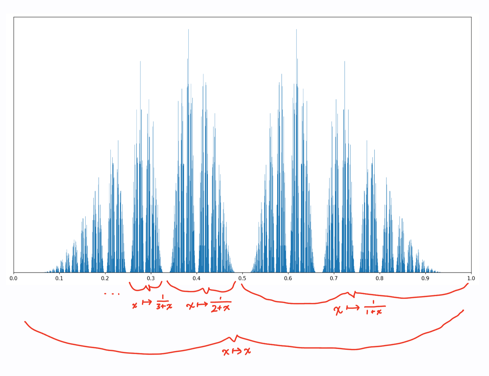
It also explains why the PDF looks so fractally: the distribution can be expressed as a weighted mixture of many copies of itself, where each copy is constructed via a homeomorphism from \([0, 1]\) to a subinterval (though none of the transformations are affine, which is why the PDF isn’t self-similar like a true fractal). For example, 50% of the probability mass comes from words that start with X — this corresponds to the homeomorphism \([0, 1] \stackrel{\small x \mapsto \frac{1}{1 + x}}{\longrightarrow} [\frac{1}{2}, 1]\). The next 25% of the probability mass comes from words starting with OX; this is given by the homeomorphism \([0, 1] \stackrel{\small x \mapsto \frac{1}{2+x}}{\longrightarrow} [\frac{1}{3}, \frac{1}{2}]\), and so on.
Minkowski’s Question Mark Function
ChatGPT helpfully informed me that this limiting distribution, though not this particular problem, has been studied before as the measure induced by Minkowski’s question mark function. The question mark function is obtained by taking the continued fraction sequence of a real number and interpreting it as the run-length encoding of a binary representation. This encoding is slightly different from the one we used to solve this problem — in particular, it makes the function monotonic:
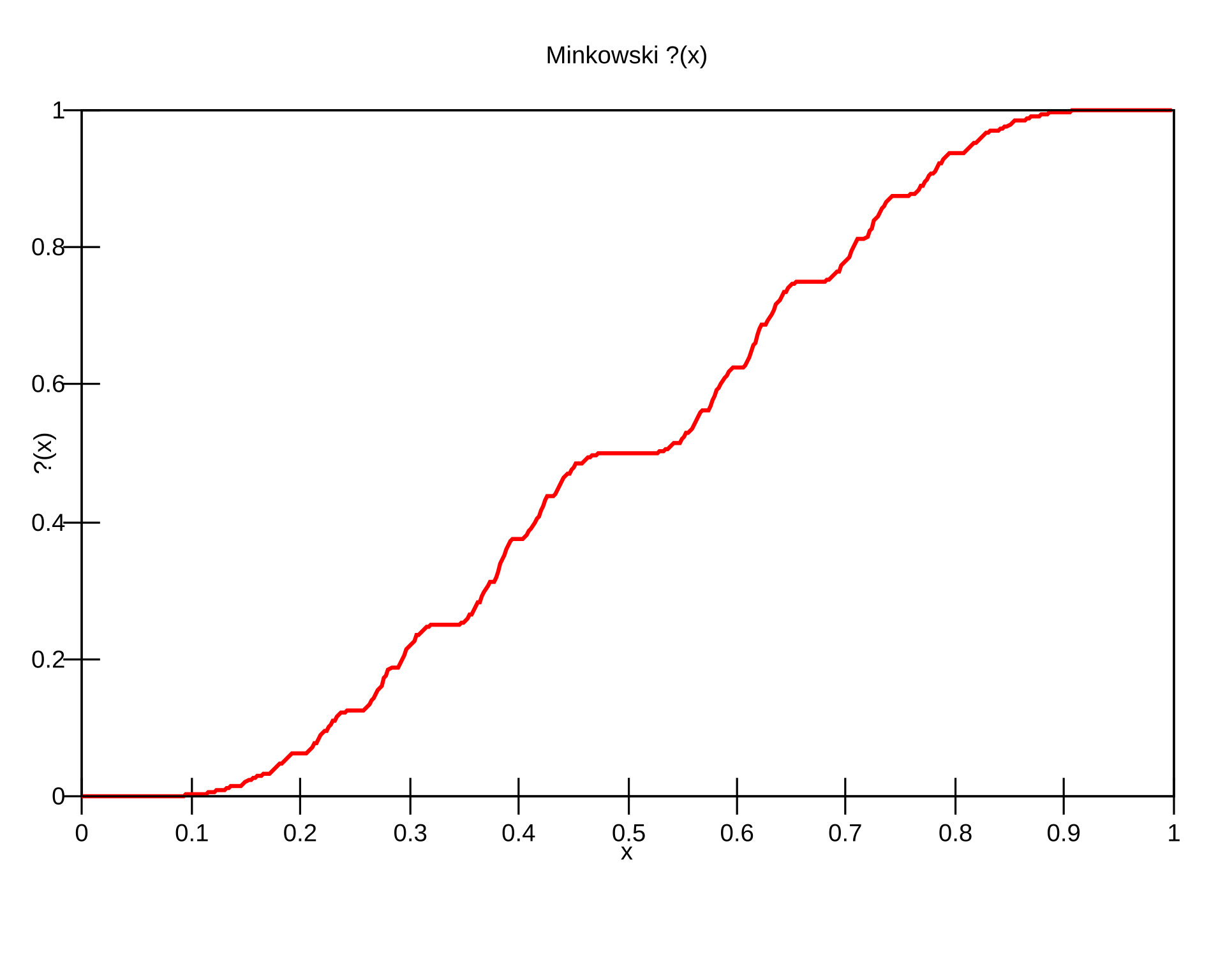
Source: Wikipedia.
Thanks for reading!
-
GPT-5 Pro can also solve this problem in ~10 minutes. ↩
-
Technically, the distribution has infinite density at these locations, so the “maxima of the PDF” (and even the PDF itself) isn’t well-defined. But we can still talk about which points have the fastest growing density, in the sense of the \(x\) at which \(\Pr[\mid \!\! X-x \!\! \mid < \epsilon]/\epsilon\) grows the fastest asymptotically as \(\epsilon \to 0\). ↩